Simulating a TRON Transaction's Gossip Trace from Public Listener IPs
A TRON transaction spreads by gossip the way a rumor does in a crowded room, each listener tells the nearest peers, they pass it on the same way, and within milliseconds the wave has reached everyone still connected through that relay pattern. Which makes a strange question answerable from the outside. If the rule is "tell the people closest to you," and we can see exactly where every listening machine on TRON physically sits, because TronScan publishes the IPs, then we should be able to draw the rumor. We have a list of IPs with latitudes and longitudes, one equation that turns two coordinates into a distance in kilometers, and a breadth-first walk outward from whichever machine we declare as patient zero.
The rest of this post is about why it works at all, what a raw listener IP is really telling us the moment you pair it with a coordinate, and why the mathematics hiding under the three-line simulator (random geometric graphs, haversine geodesics, BFS wavefronts on a metric space) is the quietly beautiful part.
What follows, in short.
- The dataset: a public list of TRON node IPs
- The question that makes the IPs useful
- The graph, in one equation
- Gossip as BFS on a geometric graph
- Why this is mathematically interesting
- What the simulator actually produces
- What this is
The dataset: a public list of TRON node IPs
The input is a flat list of TRON listener IPs. It comes from TronScan's nodemap HTTP endpoint at https://apilist.tronscan.org/api/nodemap, which returns every listening node TronScan has observed on the public network along with its geolocation.
The fetch step in this repo is fetch_tron_nodes.py: it calls nodemap/client.py for the HTTP GET, then normalizes the varying field names the endpoint returns (ip/host/address, lat/latitude, etc.) into five clean columns — IP, city, country, latitude, longitude — and writes tron_nodes.csv beside the script (generated; not committed). That CSV is the only input to the entire simulation. No private relays are consulted, no running node is instrumented, and no peer table from any real TRON client is read at any point.
One row per listener, one listener per row. Three of them from the top of the file:
ip,city,country,latitude,longitude
1.160.12.14,Taipei,Taiwan,25.0504,121.5324
1.160.151.1,Beimen,Taiwan,23.2663,120.1221
1.160.20.51,Taipei,Taiwan,25.0504,121.5324
That is the sum total of the public knowledge this post uses about the TRON network. Everything below is built on top of those five columns.
The question that makes the IPs useful
A raw listener IP looks like a fact about infrastructure. The moment you pair it with latitude and longitude, it becomes a fact about geography, and geography is the one feature of a P2P network that anyone can reason about from the outside. Peering policies are private. Latency tables are private. Super representative topology is semi-private. But where a machine physically sits is observable, and physics still insists that a signal between two boxes spends at least distance / c seconds in flight.
So the thought experiment is: if gossip obeyed distance alone, what shape would a transaction trace take?
That question sounds naive until you try to answer it. The result is a spanning tree rooted at the origin, with layers, choke points, and isolated islands laid out as a map of potential wavefronts you can scan visually.
The graph, in one equation
Build an edge between listener i and listener j if and only if the great-circle distance between them is at most some threshold link_km. The great-circle distance on a unit sphere between two points at latitudes φ₁, φ₂ and longitudes λ₁, λ₂ is the haversine formula:
a = sin²((φ₂ − φ₁)/2) + cos(φ₁) · cos(φ₂) · sin²((λ₂ − λ₁)/2)
d = 2R · asin(√a)
with R ≈ 6,371 km. Compute this for every pair, threshold at link_km = 800, and you have an unweighted, undirected graph. Only pairwise great circle distance against link_km feeds the adjacency rule, which rolls ISP paths, AS paths, ports, and RTT into that single distance gate.
The matrix of pairwise distances is n × n and symmetric, so for 7,638 nodes that is about 29 million upper-triangular entries. Cheap in NumPy. The adjacency matrix is just D ≤ link_km, which collapses the whole physical-layer story into a single Boolean tensor. The code path is gossip/geo.py (haversine_matrix_km).
Gossip as BFS on a geometric graph
Propagation now becomes breadth-first search. The origin sits at hop 0. In round r, every unvisited node that shares an edge with at least one hop-(r−1) node gets added at hop r, and we record the closest hop-(r−1) neighbor as its canonical parent (keeping the runners-up in a candidates list for ties). The recursion ends when the frontier is empty. The implementation is gossip/simulate.py (simulate_gossip).
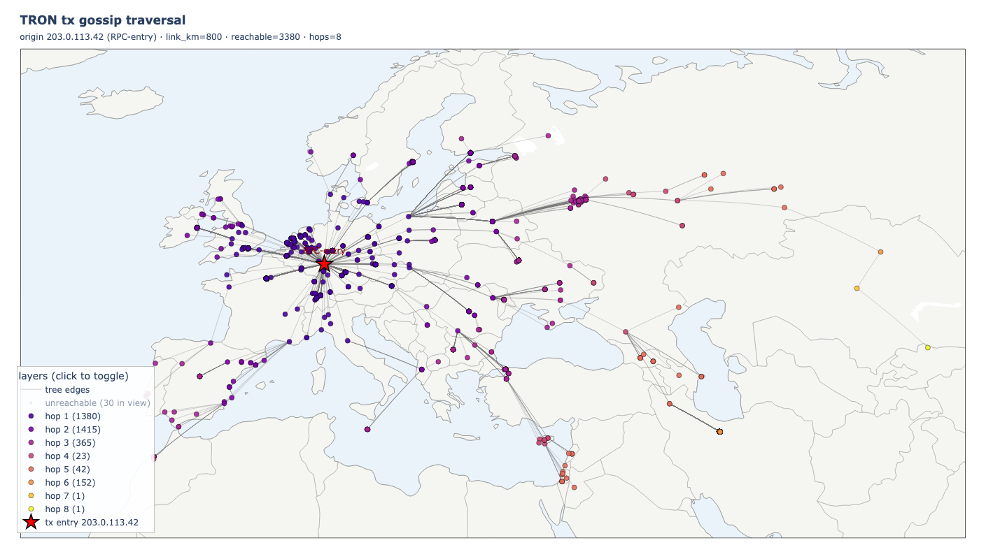
In the bundled run the histogram tells the whole story:
hop 0 :      1
hop 1 :  1,380
hop 2 :  1,415
hop 3 :    365
hop 4 :     23
hop 5 :     42
hop 6 :    152
hop 7 :      1
hop 8 :      1
Two observations are immediate. First, the first two hops cover 73% of everything that will ever be reached, which is a rate of expansion that is characteristic of geometric random graphs with dense local clusters. Second, the thin waist at hop 4 (only 23 new nodes) is a real geographic chokepoint, a narrow corridor of listeners that has to be traversed before the wave can spill into the next regional cluster. Hop 6 then balloons back up because the wave has popped into a new basin. You can see this on the map as a Central-Asian or Middle-Eastern bridge.
The 4,258 nodes that stay off the trace in this run are unreachable from this origin at link_km = 800. They are on islands, meaning connected components that lie outside the origin's component under the 800 km threshold. Change the origin or raise the threshold and the islands merge.
Why this is mathematically interesting
Start from the construction. You place one point per listener on the sphere. You draw an edge when great-circle distance (haversine distance) is at most link_km. That object is a random geometric graph (RGG): vertices live in a metric space, and geometry alone decides adjacency.
Classical RGG theory studies the clean case where n points are spread at random through a bounded region. Pairs within distance r get edges. There is a sharp percolation phenomenon. Below a threshold radius, components stay small. Above it, a giant component appears: most points can reach each other through edges. A standard scale for the threshold is r_c ~ √(log n / n).
The TronScan nodemap is not that idealized draw. Listeners pile up in Frankfurt, Tokyo, Singapore, Virginia, and other hubs. Dense pockets behave as if the threshold were lower there. Sparse oceans behave as if it were higher. So link_km is not a magic constant from a textbook. It is a dial you turn on this point pattern. Raising or lowering it moves you along a percolation-style picture for this map.
Now add time in discrete rounds. Breadth-first search is the propagation rule. Hop 0 is the origin. Hop r adds every unvisited node that touches the hop r − 1 frontier. Edges still mean “within link_km on the sphere.”
Each hop can only advance the wave by about one edge length. After r rounds, every reached node lies within geodesic graph distance r of the origin. In the continuous picture, that sits inside a ball of radius about r · link_km around the entry point. Most of that ball is empty ocean. The rest is land: clusters of listeners.
The hop counts in the histogram are a coarse readout of that geometry. They behave like a binned version of “how many listeners fall near distance r · link_km from Frankfurt,” with r running over integers. Clustering smooths the curve. The thin waist at hop 4 is a place where the wave had to squeeze through a narrow geographic channel.
In one line: coordinates turn the table into an RGG; BFS turns reachability into discrete time; the map and the histogram show where the mesh is thick enough to carry a signal at a given hop budget.
Doing all of this gives us a mapping of each node's path: hop by hop, who relayed to whom.
What the simulator actually produces
You end up with three views of the same run. There is a trace table: one row per reached listener with hop, place name, parent, distance to parent, and tie hints so the tree is auditable. There is a short text report: hop counts and a few header lines about the graph size and parameters. There is a map: listeners colored by hop, edges along the chosen parents, and a marker for the synthetic entry point. Files land next to the driver; prefixes are set in code.
trace_gossip.py is the driver. It loads the nodemap spreadsheet, appends one synthetic origin row, reads link_km and coordinates from constants, calls the library, then hands results to the writers and the plotter. Edit those constants and rerun to move the entry point or tighten the link distance.
gossip/simulate.py implements simulate_gossip. It thresholds the haversine matrix, runs the synchronous BFS, and returns hop labels, parent choices, parent distances, candidate lists, and the per-round bookkeeping the other modules consume.
gossip/outputs.py serializes the trace to a flat table and the rounds to plain text. Both functions only format and write; they do not change the graph logic.
gossip/interactive.py builds the Plotly figure: layered markers by hop, optional unreachable listeners in grey inside the viewport, tree edges, hover fields for IP and geography, and browser or pickle output depending on flags passed from the driver.
What this is
It is a thought experiment made computational. It lets an investigator or a reader look at a nodemap and see which parts of the network are dense, which parts are bridges, which parts are isolated, and how many hops it would take for a message to cross from one cluster to another if gossip respected only geography. That is a useful mental model and a good sanity-check on top of the raw table.
The shipped code path implements geographic BFS on the public nodemap. A full production stack adds peering policies, inventory scoring, fanout caps, NAT, and super-representative placement for live gossip on top of the real mesh. Every generated file still carries the toy disclaimer in its header.
The open question is how much of a P2P network's behavior first principles can recover from public IPs and coordinates alone. The simulator gives one concrete answer on that curve, and pairing that output with production traces shows how much behavior still lives in those extra layers.